

Relative entropy is a really cool tool that which haven’t heard of before you are in for a treat! Also known as Kullback-Leibler divergence, it is the measure of the distance between 2 probability distributions [e.g. p(x) and q(x) ] on a random variable X. It is defined as:


Where H(P,Q) is the cross entropy of P & Q and H(P) is the entropy of P. Note: the the log is taken as base 2 if info is measured in unit bits or base e if in unit nats.
It is called entropy because it is related to how p(x) diverges from the uniform distribution on the support of X. The more divergent it is, the larger the relative entropy.
Just like the scientific term of entropy, it is always non-negative and zero entropy means that the 2 distributions are a perfect match.
Note that Relative Entropy is *not* always symmetric! 
For 2 gaussian distributions, we can write relative entropy in the following way:
![D(P_2||P_1)=\frac{1}{2}[(\frac{\mu_1-\mu_2}{\sigma_1})^2 + (\frac{\sigma_2}{\sigma_1})^2+2\log(\frac{\sigma_1}{\sigma_2}) -1]](https://s0.wp.com/latex.php?latex=D%28P_2%7C%7CP_1%29%3D%5Cfrac%7B1%7D%7B2%7D%5B%28%5Cfrac%7B%5Cmu_1-%5Cmu_2%7D%7B%5Csigma_1%7D%29%5E2+%2B+%28%5Cfrac%7B%5Csigma_2%7D%7B%5Csigma_1%7D%29%5E2%2B2%5Clog%28%5Cfrac%7B%5Csigma_1%7D%7B%5Csigma_2%7D%29+-1%5D&bg=ffffff&fg=7f8d8c&s=0&c=20201002)
For a d-dimensional Multivariate normal:

Example Normal distributions:
Let’s make some toy data of 2 gaussian distributions and calculate their relative entropy.
rel_entropy<-function(mu1,sigma1,mu2,sigma2){
 #returns D(P1||P2)
 out=0.5*(((mu1-mu2)/sigma1)^2.0+(sigma2/sigma1)^2.0+2.0*log2(sigma1/sigma2)^2.0-1.0)
 return(out)
}
options(repr.plot.width = 10, repr.plot.height = 6)
par(mfrow=c(1,2))

#first pair of gaussians will vary in mean
m1=0
s1=1
m2=2.3
s2=1
x=seq(-3,3,0.1)
D1=rel_entropy(m1,s1,m2,s2)
plot(c(-3,3),c(0,1), ty='n', xlab = 'x', ylab = 'p(x)', main=paste('D(p1||p2)=', format(D1,digits = 2),sep=''))
lines(x,dnorm(x=x,mean = m1,sd =s1 ), col='sky blue', lwd=3)
lines(x,dnorm(x=x,mean = m2,sd =s2 ), col='pale green',lwd=3)
legend('topleft',legend=c(expression(p[1]*' : '*mu[1]*'=0, '*sigma[1]*'=1'),expression(p[2]*' : '*mu[2]*'=1, '*sigma[2]*'=1')), col=c('sky blue', 'pale green'), lty='solid', bty='n', lwd=3)

#second pair of gaussians will vary in standard deviation
m1=0
s1=1
m2=0
s2=0.5
x=seq(-3,3,0.1)
D1=rel_entropy(m1,s1,m2,s2)
plot(c(-3,3),c(0,1), ty='n', xlab = 'x', ylab = 'p(x)', main=paste('D(p1||p2)=', format(D1,digits = 2),sep=''))
lines(x,dnorm(x=x,mean = m1,sd =s1 ), col='sky blue', lwd=3)
lines(x,dnorm(x=x,mean = m2,sd =s2 ), col='pale green',lwd=3)
legend('topleft',legend=c(expression(p[1]*' : '*mu[1]*'=0, '*sigma[1]*'=1'),expression(p[2]*' : '*mu[2]*'=0, '*sigma[2]*'=0.5')), col=c('sky blue', 'pale green'), lty='solid', bty='n', lwd=3)
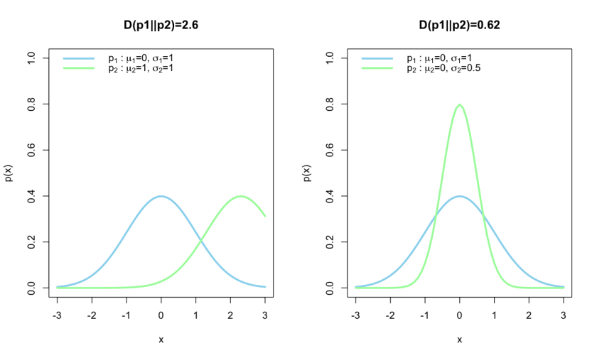
On the left plot we see that given the gaussian p2, the entropy is quite large, and since entropy is a measure of the gain in information, we can say that there is a large gain in information. On the the other hand the plot on the right has a lower relative entropy. We expected p1 to give us tighter constraints than p2 so that fact that the posterior got broader shows the information gain from p1 given p2 is smaller.
Now reversing p1 and p2 in the relative entropy calculations results in the following plot:
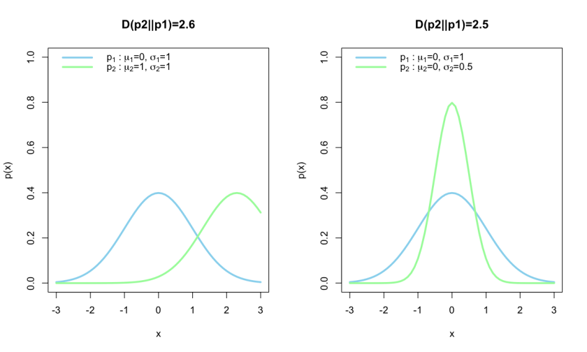
Notice that in the left plot, the reversal has no effect on the entropy, since the amount of information gain is the same, whereas on the right hand side the entropy has increased much more, the amount of entropy is larger because we obtained tighter constraints on the posterior and thus gained a lot of information.
Surprise
Now relative entropy is all well and good, but it doesn’t really tell us much on its own. This is where Surprise comes in. Surprise S is given by the Relative entropy minus the expected relative entropy and is a measure of tension.
where
is the expected relative entropy, usually given as the mean of the prior distribution of


![= \int \left[\int p(\Theta|D_1)p(D_2|\Theta)d\Theta\right] D(p(\Theta|D_2)||p(\theta|D_1)) dD_2](https://s0.wp.com/latex.php?latex=%3D+%5Cint+%5Cleft%5B%5Cint+p%28%5CTheta%7CD_1%29p%28D_2%7C%5CTheta%29d%5CTheta%5Cright%5D+D%28p%28%5CTheta%7CD_2%29%7C%7Cp%28%5Ctheta%7CD_1%29%29+dD_2&bg=ffffff&fg=7f8d8c&s=0&c=20201002)

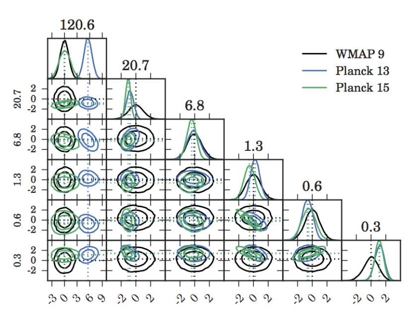
Now the paper Seehars+2016 is a good demonstration of these 2 tools in action. In their paper they look at the tensions between the cosmological parameters measured by 3 different CMB (see here for a review) survey results, WMAP9, Planck2013 and Planck2015.
In their paper they show that the marginalised posteriors of cosmological parameters from the Planck2013 team seem to be more in agreement with those of Planck2015, and in tension with those of WMAP9.
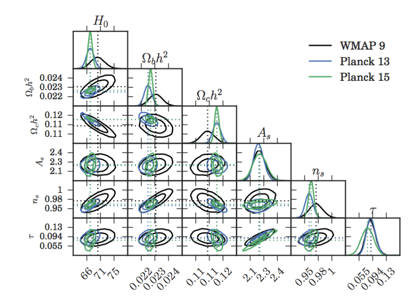
Seehars+2016 Fig 2. 1D and 2D marginalised posteriors of the cosmological parameters
However on their analysis of Relative entropy and Surprise, they actually found better agreement between WMAP9 and Planck2015. Remember surprise is a measure of tension. The relative entropy was small, but the surprise was negative, which means they were not at all surprised at the Planck2015 results given the WMAP9 results.
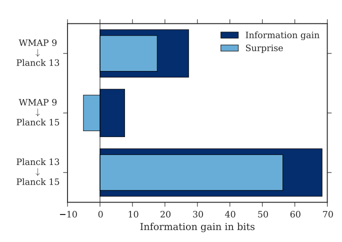
Seehars+2016 Fig 1. Relative entropy and surprise of results from various CMB surveys
From this, they do a PCA analysis and find that whilst in the given marginalised posterior spaces the Planck results are in better agreement, re-parameterising in terms of eigenvector spaces with the largest eigenvalues, they find WMAP9 and Planck2015 to be in better agreement.
Seehars+2016 Fig 4. 1D and 2D marginalised posteriors under the new parameterisation.
